If you have worked with inferential statistics, you’ve certainly heard of a p-value. You likely also have heard about the pushback against p-values. Effect sizes become part of the conversation when looking to move beyond a singular overreliance on p-values. A p-value describes how incompatible the data are with a specified statistical model, but it does not show how large a difference or relationship is. An effect estimate describes that magnitude. A confidence interval describes its precision. Whether the effect is large enough to matter requires context and a decision threshold.

Effect sizes may sound easy enough to pick up and use alongside your p-values. However, while effect sizes might be slightly more intuitive than p-values in their output, they also have more points in the decision tree when implementing them. Reading through some papers, I found that some widespread guidance (and what I previously thought) is not quite right. I want to spend a couple (or maybe a few) posts sharing what I’ve learned. You should be using effect sizes in statistical results, but it’s important to do them correctly. 

The basics

First I’ll touch on the concepts of p-values and effect sizes. We need to know the basics before we can deconstruct our decisions around effect sizes. Effect sizes and p-values answer different questions, so I’ll start with p-values. If you know all this already, just jump to the recommendations around effect sizes.

P-values

One of the core frequentist tools for statistical models is the p-value, but it is poorly understood. I’ve seen lots of discourse in UX research lately that we must focus on effect size as a cure for the woes of using p-values. Lots of the discussion I’ve seen on LinkedIn or blogs is well-intentioned but is fundamentally inaccurate. I’ve seen calls to ignore the p-value entirely. It would be odd to report an effect estimate in a confirmatory project without also reporting inferential uncertainty. Here, the p-value shows how compatible the data are with the null hypothesis under the model, while the confidence interval shows the estimate’s precision.

So what is a p-value? The precise definition of a p-value is:

The p-value is the probability, computed under the assumption that the null hypothesis and all other model assumptions are true, of obtaining a test statistic at least as extreme as the one observed.

If that left you more confused, jump to my in-depth explainer. 

In addition to the definition, I want to draw your attention to a few key points from the American Statistical Association about what p-values do and do not do.

“P-values can indicate how incompatible the data are with a specified statistical model.”

This is important because it states the original value a p-value brings and why we should not discard it. But on its own, it’s insufficient.

“Scientific conclusions and business or policy decisions should not be based only on whether a p-value passes a specific threshold.”

“A p-value, or statistical significance, does not measure the size of an effect or the importance of a result.”

We must turn to effect sizes to help guide us to understanding the importance or strength of the variable relationships we care about in our models.

Effect sizes

Effect sizes are the statistical tool most commonly used to move beyond simple compatibility of data with a statistical model (statistical significance) and into practical significance. Psychology’s reporting guidance has emphasized effect sizes for decades. In 1999, Wilkinson and the American Psychological Association’s Task Force on Statistical Inference recommended reporting effect-size estimates for primary outcomes. The need for effect sizes in applied, business contexts is even more evident because teams often prioritize the concept of practical significance to a decision at hand, not broader implications for a grand scientific truth.

The precise definition of an effect size is not as clear-cut as that of a p-value. Kelley and Preacher have a good review of other definitions and provide this definition that I will use:

“Effect size is defined as a quantitative reflection of the magnitude of some phenomenon that is used for the purpose of addressing a question of interest.”

If that left you more confused, MeasuringU has a great introduction to effect sizes. 

There is not much discussion of p-values in the UX research domain, perhaps because the field is so applied or traditionally qualitatively focused. There is even less discussion of effect sizes, despite their importance in modern statistical approaches. However, effect sizes are crucial to making good use of statistical models in applied decisions.

That was a lot of fundamentals to cover, even in abbreviated format, before getting to the real substance of this post: how you should use effect sizes in your work. As I wrote this out, I realized I needed to break it up into pieces, so I am going to start with calculating effect size the right way, and part II will cover how to decide what is big or small in an effect size.

The right effect size calculation

As mentioned above, MeasuringU has the post to read for getting up to speed on effect sizes in UX research. It gives a broad overview, and, perhaps intentionally for that reason, maintains a somewhat unopinionated view on a couple key points in application. While they cite a paper by Funder and Ozer in their post, I want to draw even more out of it than they did for our application in UX research. It also has a great title, “Evaluating Effect Size in Psychological Research: Sense and Nonsense”. 

This academic paper takes a very opinionated view, if you couldn’t tell that from the title alone, on reporting standardized vs. unstandardized effect sizes. In psychology domains, effect size often is shown in standardized format, typically Cohen’s d (the difference between two group means divided by their pooled standard deviation). An unstandardized effect size skips that division and reports the difference in the unit you originally measured it in (e.g., 17 seconds, 9 percentage points, 0.4 scale points).

First, we have to mention where standardized effect sizes work well.

• Some power analyses use standardized effects. Others use a target difference and assumed variability in the original unit.
• Standardization can help when a comparison combines measures with different units, such as some meta-analyses or within-study comparisons.
• When a reader will have no context for a measure and won’t need it for the future (like a bespoke composite), there is some argument for the standardized effect size.

There are other arguments for standardization that I will argue don’t outweigh the negatives, particularly when a measure has an arbitrary value (like a Likert scale). So outside of the cases I mentioned, which are mostly rare for a UX researcher, you should be using unstandardized effect sizes (because you should use effect sizes in general any time you use a p-value). 

Why you probably shouldn’t standardize your effect sizes

Standardization has a number of drawbacks and limitations. It is biased upward in small samples, it is not comparable between within-subjects and between-subjects designs, and different papers divide group mean differences by different standard deviations which makes them less comparable than they first appear. All of these have some workarounds (read the full paper from Funder and Ozer to dig in), but I want to focus on the primary reason you as a UX researcher should leave effect sizes unstandardized. 

Standardization removes useful context

Standardization removes discernible context from the numbers you’re dealing with. When you divide a difference between means by the standard deviation, it removes the unit from the result. There is no fix for this other than not standardizing, as that is the purpose of standardization in the first place. The unit is what researchers and stakeholders need to make decisions about the applied context at hand.

Example

Let’s imagine you have a new version of a support system that you test with 50 users per version. You measured completion time: 95 seconds on A (SD 60) and 78 seconds on B (SD 50).

With a standardized effect size you’d say, Cohen’s d = 0.31. You may describe it as small-to-medium in strength of improvement for the new design on task time. The problem is (as we’ll see in the next section) that small-to-medium T-shirt size is arbitrary.

With an unstandardized effect size you’d say, −17 seconds. This is tangible, and if you know the business context, it can be linked clearly. Say the task is done 100 times a day by support employees across 250 workdays per year. That would save about 28 minutes a day, or 118 hours per year (roughly three 40-hour working weeks).

What do you want to bring to your stakeholders? “Cohen’s d is .31 which is a small-to-medium effect size, indicating that prototype B performed moderately better” or “The effect was -17 seconds for prototype B which could save 3 working weeks per year”. 

It’s obvious here which is more helpful. Reporting unstandardized effects makes applied decisions clearer and easier to make.

Arbitrary measures and ceiling effects

What about situations where the values are arbitrary, like the Single Ease Question (SEQ)? There is less value in sharing the raw number, but standardization still causes issues particularly when there are ceiling effects or floor effects in the score. 

Ceiling effects occur when a score reaches near the upper bound of its scale (say 6+ out of 7 on the SEQ). On a bounded scale, the maximum possible standard deviation is fixed by where the mean sits. Population variance cannot exceed (max − mean) × (mean − min). The table below applies this bound to both means for a 0.4-point improvement on a 1–7 scale. For this illustration, both groups have equal weight and the SDs use population variances. The largest possible pooled SD is the square root of the average of the two variance bounds, and dividing 0.4 by that SD gives the smallest possible Cohen’s d.

Mean before	Mean after a +0.4 gain	Largest possible pooled SD	Smallest possible Cohen’s d
4.0	4.4	2.99	0.13
5.5	5.9	2.46	0.16
6.0	6.4	2.03	0.20
6.5	6.9	1.29	0.31
6.6	7.0	1.06	0.38

The denominator of d is constrained partly by where both group means sit. Even with identical gains, the minimum possible standardized effect nearly triples as the scores approach the ceiling (.13 for a gain from 4.0 to 4.4, compared with .38 for a gain from 6.6 to 7.0).

With Likert items and scales, like the SEQ, ceiling effects are common. I say this from personal experience, but there is some published evidence to corroborate my anecdata. Let’s take a look at the implications in practice.

Example

Imagine two food delivery apps. Tiffin is an average product. Skillet is a very good one. Both ask the same SEQ question after a checkout task, and both collect the same number of responses. Tiffin scores a mean of 5.0 and Skillet scores a mean of 6.4. Their standard deviations are quite different, 1.47 and 0.79. Skillet’s mean is closer to the ceiling, which lowers the largest possible SD.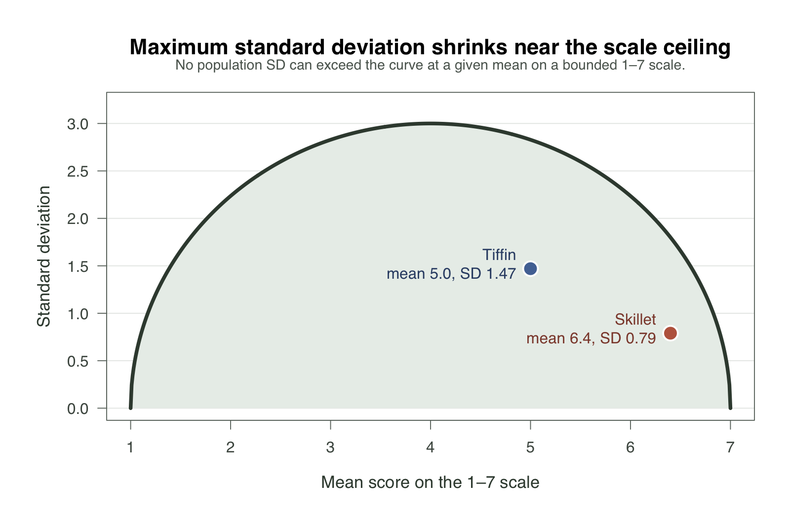

This starts to become problematic when we compare differences. Imagine both improve their SEQ by the same number, 0.4 points. For this example, assume each app’s SD stays the same after the improvement, so the pooled SDs remain 1.47 and 0.79. Tiffin’s improvement shows a Cohen’s d of 0.27, whereas Skillet’s is 0.51. With an identical gain in scale points, the standardized effect is nearly twice as large because Skillet’s SD is smaller. The ceiling artificially constrains which SDs are possible, warping our vision of the practical importance of the gain. 

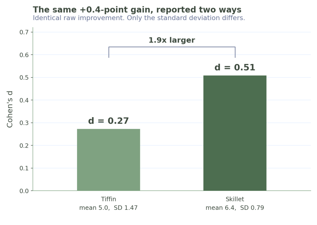
In the big picture of a measurement program, you will systematically overstate the wins on your strongest experiences and understate them on your weakest experiences. This bias is embedded into the standardization.

Likert scale effect sizes may be tempting to standardize because of the arbitrary unit argument, but Likert scales also frequently have ceiling effects. Therefore, I do not see clear reasons to rely on standardized effect scores outside of uncommon circumstances in UX research, like a meta-analysis.

Misconstrued effect sizes

One last piece that is not so much about removing useful context, but introducing an unhelpful context, is the way the number is interpreted intuitively by researchers and stakeholders alike.

If you’re a researcher and you’ve run correlations or regressions before, you’ve likely looked at a variance-explained measure for effect size and said, “Wow, this important variable only explains 9% of the variance overall.” I have done this many times in the past only to learn this way of reading the numbers is almost actively misleading.

Consider a stylized checkout example with four equally common groups that are being tested. The groups are: no upsell, upsell module A only, upsell module B only, and both upsell modules. Module A adds exactly four dollars to order value on average and module B adds exactly eight dollars on average, with no other variation. Under this constructed setup, their correlations with added order value are approximately r = .45 and r = .89. Squaring them gives 20% and 80% of variance explained. That makes module B sound four times as strong (20% vs. 80%), even though its effect in dollars is twice as large (4 vs. 8 dollars).

Even viewing standardized effect sizes alone is misleading. As a separate, deliberately simplified example, we have an r of .30 explains 9% of the variance. The authors recommend using a binomial effect-size display to compare outcomes on a 2 x 2 chart. Under the binomial effect-size display, that same correlation of .30 maps to 65% in one group versus 35% success in another. This is almost a two-to-one difference in success rates. So is an r² of 9% really that small? I don’t think so.¹

Wrap up

If you are using p-values, you should also be using effect sizes. A p-value reports how compatible your data are with a model that assumes no effect. It does not report how large the effect is, and your team cannot decide anything effectively without that information.

So, how do you report the effect size? Standardization is common. It is most useful in specific cases: some power analyses, pooling measures that do not share a unit, and measures whose original unit gives readers little context. Outside those cases it should not be your default, because of the three major problems I highlighted here.

First, standardizing removes the unit, and the unit is what a stakeholder uses to make a decision. Getting a difference of seventeen seconds in your usability benchmark relates directly to your product’s staffing and cost, whereas a result of d = 0.31 is abstract entirely.

On bounded scales such as the SEQ, it may be tempting to standardize because of the arbitrary units. However, this runs into the second problem that is common with UX Likert scales like usability or satisfaction measures. Standardizing increases the reported effect where scores already sit near the top of the scale range. The same improvement across two different groups will look artificially larger on your strongest experience and smaller on your weakest one.

Lastly, standardizing distorts how important numbers appear. For example, squaring the two correlations in the checkout example produces a 4:1 ratio in variance explained, even though the effects in dollars have a 2:1 ratio. An r of .30 can also sound small when described as 9% of the variance, while the binomial effect-size display translates it to 65% versus 35% success rates, which reads as much larger.

Given all of these issues, it’s best to report the raw difference for an effect size (and its confidence interval) in your key results. Standardized effects should be omitted outside a few rare cases in UX research.

In my read of Funder and Ozer, I picked up one other critical consideration for effect sizes. Once the effect is stated in plain units, how do you determine if it is small or large? This is the subject of the next post on effect sizes, so stay tuned.

Appendix

P-values

Jump back to context in the post

Before we get to effect size, we must discuss p-values. This is what you’re most likely to have come across. It’s what researchers talk about when they say something is “statistically significant”. Researchers often choose alpha = .05 as the significance threshold. In an ordinary two-sided test, the matching confidence interval has 95% coverage. The something which can be significant is not a single number or a sample size. There has to be some relationship to compare, whether it’s which number is bigger or how related two numbers are, at the most basic. 

P-values exist in a testing framework. 

• There is a conventional assumption (null hypothesis) that there is no effect of a predictor or difference between two groups’ values. There is also an alternative hypothesis
  • Null hypothesis = no difference in task completion times between groups A and B. Alternative hypothesis = a difference in task completion times between groups A and B. 
• Then you run the study and get your result.
  • Group A completes in 50 seconds, group B in 90 seconds.
• A p-value of 0.05 is how we ask: If we ran this study under the exact same conditions 100 times, and there was truly no difference between the groups (and all our statistical assumptions were perfectly met), we would expect to see the difference we got, or an even larger one, only 5 times.
  • Because seeing a 40-second difference is so unlikely if the groups are actually identical, you reject the assumption that they are the same. Strictly, that is all you have done: rejected one specific claim while controlling how often you would do so wrongly. It does not establish that the 40-second difference you measured is the true difference, and it does not establish that 40 seconds matters.

It’s a bit convoluted and unintuitive, but this is the precise way to think about p-values. If you look online, you will find several definitions that sound plausible but leave out an important condition: the probability is calculated under the null hypothesis and the other model assumptions. The definition above is the one I rely on here.

What do p-values not say? They do not say that our alternative hypothesis is true. They do not say the probability that the data were produced by random chance alone. And most importantly for us here, they do not say how big or important the effect or difference between groups is.

1. The binomial effect-size display assumes equally sized groups, dichotomizes the outcome, and fixes the overall success rate at 50%. It illustrates why r² can make an association sound small, but it should not replace the observed success rates when those rates are available. ↩︎