In my last post about effect sizes, I talked about what makes an effect size big or small. (Hint: it depends.) The more useful question for applied work is: Is the effect large enough to change the decision? Most of the time, UX research is run without this target number in mind. Often, clinical research studies specify an importance threshold before collecting data. For example, the minimal clinically important difference is one way researchers define a context-specific threshold of what matters when studying medical interventions.
Experts in medical fields spent lots of time researching what a big enough change is to matter across their domains. It would take a lot of work in UX research too. The effort is worth it for two reasons: it lets researchers combine statistical and practical significance in one analysis procedure, and it shows whether a study design can capture the change the team cares about.
We’ll dig into both of those and how you can arrive at your number. For our purposes, I’ll call that big enough number the action threshold. Minimal important difference is another common existing name. Important does not necessarily mean action, which is what we are most often driving in a UX research context. Another term is the smallest effect size of interest (SESOI). I find this too technical for communication with stakeholders.
I want to first cover how we use the action threshold in analysis. The next post will show how to choose it. I explain the analysis first so the requirements for a usable threshold are concrete. So, let’s get into action-threshold testing as a way to combine statistical and practical significance.
Combining statistical and practical significance
My first post on effect size covers what an effect size is and how it differs from a p-value. A p-value answers a compatibility question under a specified model. An effect estimate describes the magnitude of a difference or relationship. A confidence interval describes the estimate’s precision. The action threshold connects the estimate to a decision. Effect sizes are not something I see commonly used or well-understood across UX research right now. That said, they are quite useful.
In UX research, the only framework I’ve seen around using p-values and effect sizes in conjunction comes from Lewis and Sauro. Even if you haven’t read this, you’ve probably done something similar if you have implemented effect sizes in your work.
Broadly, their approach runs a significance test and calculates a confidence interval around the group mean difference. When the result is significant, you look at the lower limit and ask whether the smallest difference compatible with the data at that confidence level is still big enough to matter. When the result is not significant, you look at both limits and ask whether they are close enough to zero to treat the difference as zero for practical purposes.
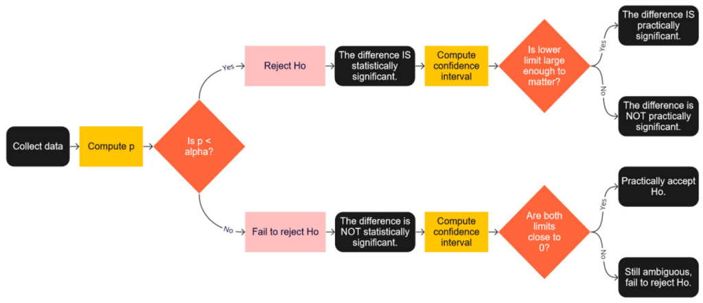
This framework is broadly correct, but a few key corrections are needed. The two big ones are (1) choosing an action threshold before you run the study or models and (2) properly structuring equivalence and minimum-effect tests. Choosing an action threshold requires a post all its own, so we’re going to start with number 2. This means we assume we already have our action threshold chosen, the smallest difference the team will act on, and dig into the modeling approach that combines statistical and practical significance.
No evidence of an effect is not evidence of no effect
When you test something, say two groups on the SEQ or two reported behavior frequencies, you’re typically testing whether there is a significant difference between the groups or responses. In a test of significant difference, this is our alternative hypothesis (H1): there is a difference between the groups. The null hypothesis (H0) is that the difference between the groups is exactly zero1.
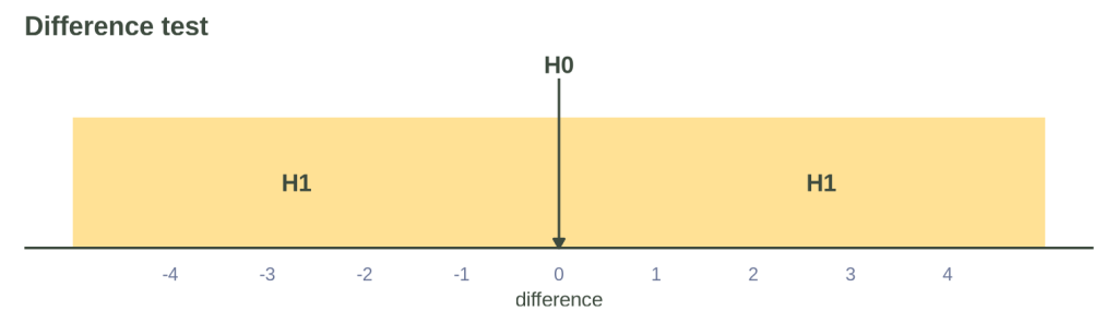
A test of significant difference is built to reject H0, but it has no way to accept H0, such as saying the groups are the same. An intuitive error is to consider groups the same when the result is not statistically significant. Two groups that fail a difference test have not thereby been shown to be equivalent. This requires a separate equivalence test.
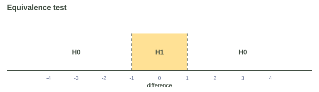
The equivalence null hypothesis contains effects at or below the lower bound and effects at or above the upper bound. The alternative hypothesis contains effects between the bounds. A finite sample cannot establish exact equality at zero. Equivalence testing asks whether the data exclude effects outside a prespecified interval around zero.
To apply this, you could use the action threshold to set the equivalence bounds. The alternative says the difference is small enough that it would not change a plan or decision.
This equivalence test asks whether the difference between your groups is small enough to be treated as the same for the decision at hand. What about when you want to say the groups differ by enough to matter, beyond simply being different at all?
Minimum-effect testing puts the action threshold into use
A minimum-effect test evaluates the complementary claim to the equivalence test: whether an observed difference is large enough to cross the action threshold.
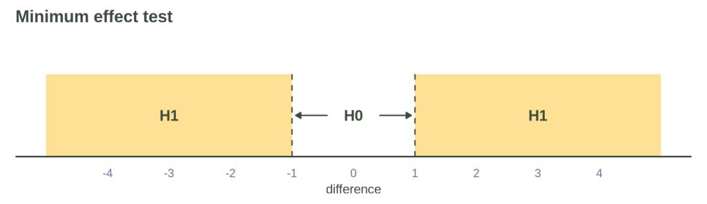
If your head is starting to spin a bit, let’s consider this in action. The minimum-effect test gives the null hypothesis (H0: a near-zero change) a range. The null covers the interval from the lower action bound to the upper action bound instead of a single point at 02. We ask whether the data exclude effects inside those bounds. In this way, the minimum-effect test is a difference test with a widened H0 (no difference -> difference small enough not to matter) when we visualize the transition between the a different test and a minimum-effect test.
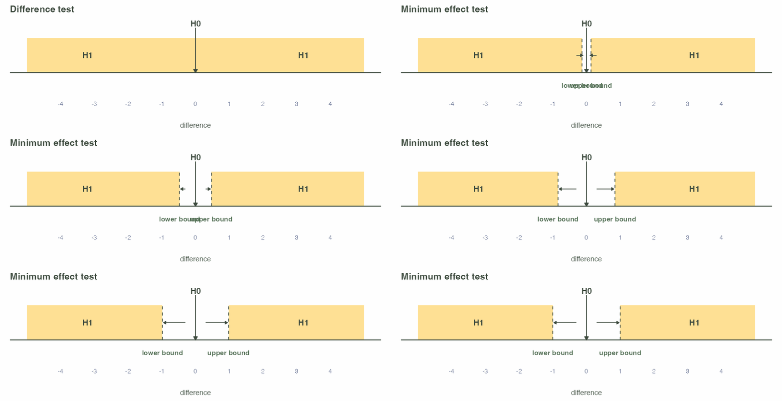
Lakens shows how the formal minimum-effect test joins statistical and practical significance in one decision rule. The value we test against represents the smallest effect worth acting on. Rejecting effects inside the bounds at least establishes that the effect crosses the action threshold under the model.
It’s also worth noting that the equivalence test is actually two one-sided tests (TOST). A two-sided minimum-effect claim uses the ordinary 95% interval at alpha .05.
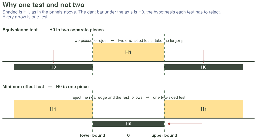
Both tests use the same action threshold:
- Equivalence testing asks whether the data exclude effects at or beyond the bounds.
- Minimum-effect testing asks whether the data exclude effects inside the bounds.
There is a third variant called a non-inferiority test. It has one bound instead of the two in an equivalence test. A non-inferiority test asks whether the data exclude effects worse than the lower margin. This would apply especially well to something like testing a redesign. The team wants to ship it, so we’re mainly concerned that it didn’t break anything (doing worse), not if it’s better. The team will want to launch even if it has the same UX quality as the current design. I’ll dig into this more in an upcoming post.
Updating Lewis & Sauro’s approach
Lewis and Sauro’s framework is quite useful and has been the clearest guidance our field has had for combining statistical and practical significance. However, the approach lacks three elements used in action-threshold testing: pre-specified bounds, formal equivalence hypotheses, and an interval matched to alpha.
1. No action threshold is chosen beforehand
The Lewis and Sauro approach does not choose an action threshold beforehand. What is big enough or small enough is chosen in each decision branch after the data are collected.
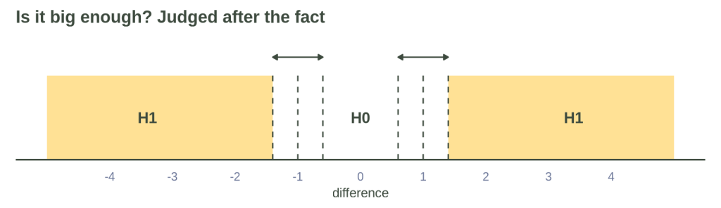
Their upper branch resembles the question answered by a minimum-effect test. When p < .05, they ask whether the lower confidence limit is big enough to matter. A formal minimum-effect test adds an explicit bound chosen before the result. The dotted lines in the plot below represent the prespecified bounds missing from the original framework.
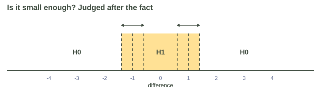
Their lower branch resembles the question answered by an equivalence test. When p >= .05, they ask whether both limits are close enough to zero. A formal equivalence test adds explicit bounds chosen before the result. Again, the dotted lines represent the prespecified bounds missing from the original framework.
What is the problem with deciding after the fact? Lakens and colleagues write, “If the bounds chosen are based on the observed data, an equivalence test becomes meaningless.”
Lewis and Sauro do not claim to run an equivalence test, so the criticism doesn’t directly apply to their approach. However, it exposes that the post hoc equivalence judgment has no prespecified Type I error rate. The confidence interval retains its ordinary coverage. The label cannot be given an alpha retrospectively because the result has already shaped what “close enough to zero” feels like.
The formal tests in action-threshold testing add a bound and error rate chosen before the result3. This is not about accusing any researcher of bad-faith judgment, but we’re all biased by how badly we want certain results to come out. Choosing the action threshold a priori helps reduce the influence of our own preferences.
2. The hypotheses are labeled incorrectly on the lower branch
The second issue is theoretically important, but a bit pedantic in application. That said, I will cover it here for thoroughness.
Their procedure does not formalize the small-enough question as an equivalence test. The lower branch treats a nonsignificant difference test as support for equivalence. On the lower arm of their decision tree, what is really a second alternative hypothesis is still labeled H0.
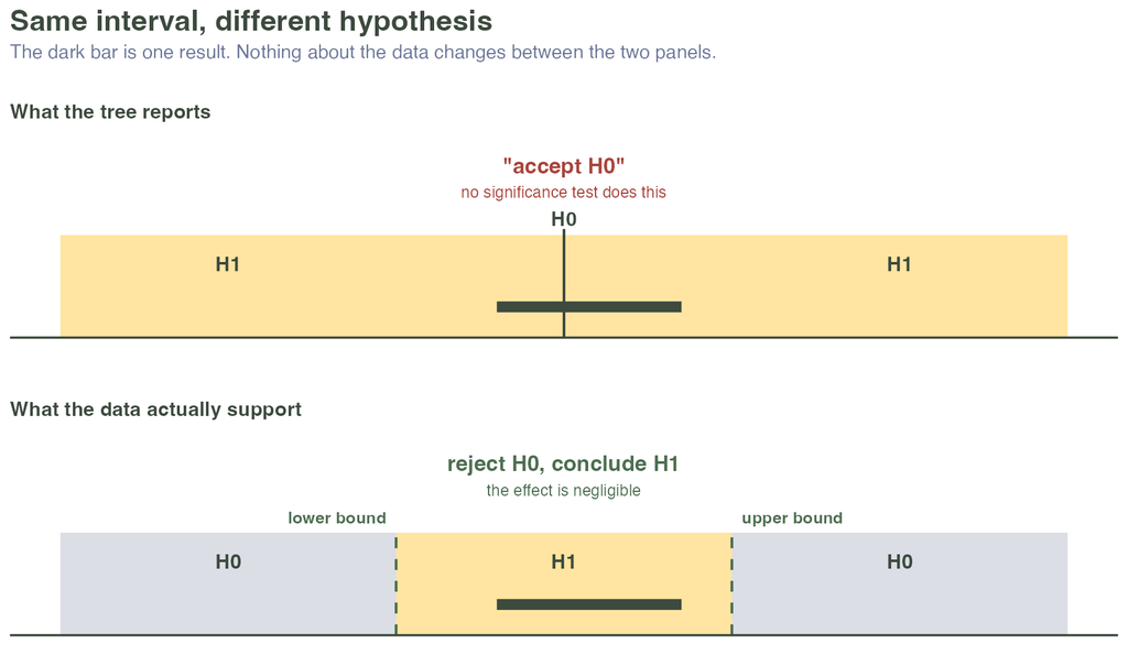
The label treats the interval as small enough without a prespecified bound or error rate for that judgment.
3. The interval is the wrong width
The last piece is narrow but easy to fix. Lewis and Sauro use a 95% confidence interval throughout. A formal TOST procedure contains two one-sided tests at alpha .05. Both tests must reject the null hypothesis, so the corresponding central interval has 90% coverage.
This means the Lewis and Sauro approach is more conservative than TOST at alpha .05. The 90% interval avoids the extra conservatism without inflating the error rate.
Action-threshold testing
We’ve identified the goal of a single procedure for statistical and practical significance, as well as the errors in existing frameworks. How should this work after adding prespecified bounds and the formal tests? I’ll call the full procedure action-threshold testing. We are covering the analysis phase, and the next article will back up to the first phase of choosing the action threshold. For now, let’s assume we know the smallest difference the team cares about.
The statistical phase uses three-sided testing (TST), an extension of what we’ve already talked about above. Isager and Fitzgerald describe TST as a combination of TOST and minimum-effect tests. TST tests whether the effect sits below the lower bound, inside the bounds, or above the upper bound. It yields inferiority, equivalence, superiority, or an inconclusive result. We also use a two-sided test against zero (and collapse the direction of positive or negative) to produce five evidence patterns for this UX decision. We’ve covered a lot already, so let’s see what we’re aiming for before we do an example.
Outcomes of action-threshold testing
When we combine TST with a two-sided test against zero, there are five possible outcomes:
A. The 95% interval sits entirely beyond an action threshold. The data exclude zero and effects inside the action bounds.
B. The 95% interval excludes zero and crosses an action threshold. The data exclude zero, and this study cannot say which side of the threshold the effect is on.
C. The 95% interval excludes zero, and the 90% interval sits entirely inside the action bounds. The data exclude zero and effects at or beyond the threshold.
D. The 95% interval includes zero, and the 90% interval sits entirely inside the action bounds. The data exclude effects at or beyond the threshold, while zero remains unresolved.
E. The 95% interval includes zero, and the 90% interval crosses an action threshold. The result remains inconclusive.
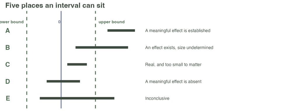
TST alone produces four directional conclusions: superiority, inferiority, equivalence, or inconclusive. I collapse superiority and inferiority into outcome A (both lead to action), then use the two-sided zero test to split equivalence into C and D and inconclusive into B and E. Lewis and Sauro merge B and C because their upper branch inspects only the lower confidence limit. In action-threshold testing, B means the data exclude zero while the threshold status remains unresolved (some effect, though unclear if big enough).
| The interval | Plain language | L&S label | Error | |
| A | 95% interval beyond ±threshold | Difference beyond the threshold is established | Practically significant | Practical label chosen post hoc; no prespecified Type I error rate |
| B | 95% excludes zero; crosses ±threshold | The redesign is better than the original, but threshold status is unresolved | Described rather than named. Their Example 2 gets “casts a shadow on the practical significance.” | Merged with C. This branch inspects only the lower limit, so the tree cannot see whether the upper limit clears the threshold, which is the only thing separating the two. |
| C | 95% excludes zero; 90% inside ±threshold | The redesign performs better than the current design, and the data exclude effects beyond the action threshold | Same description as B | Merged with B. A definite finding gets the same words as a study that couldn’t tell. |
| D | 95% includes zero; 90% inside ±threshold | Effects beyond the threshold are excluded; zero is unresolved | Accept H0, treat as effectively zero | The lower branch labels this H0, although equivalence rejects a second null in favor of a second alternative. |
| E | 95% includes zero; 90% crosses ±threshold | Zero and threshold status are unresolved | Inconclusive | No issues |
Simple worked example with SUS
Let’s see it in action to make it more concrete. As a reminder, our goal is a consistent way to read an effect estimate against zero and against a decision boundary. The pre-specified rules control the familywise Type I error for one relationship and make the decision reproducible.
Note that this error control applies to one prespecified relationship. We’ll return to multiple-testing corrections in a later worked example, where a multiple-select question creates several related comparisons.4
We will compare simulated SUS scores from a current version of an app and a redesign. Imagine the team has decided they need to act when the redesign improves SUS by at least 8 points at alpha .05. We’re going to show how to run it in base R to expose the logic more deeply. This example follows the common practice of modeling SUS as approximately continuous.
The first thing we do is get our data and run the difference test between groups. A t-test is common in the literature and will be our example, but TST can be used whenever the fitted model supplies an estimate and standard error with a justified normal or Student-t reference distribution5. For the t-test, we need:
- The test’s estimate of the difference
- The standard error
- The degrees of freedom
We then extract the difference estimate and a 95% interval and a 90% interval from the same estimate and standard error6. TOST contains two one-sided tests at alpha .05. Both must be rejected, so the corresponding central interval has 90% coverage.
Here’s how we run the three comparisons using one estimate and standard error against three reference values: zero, the lower action threshold, and the upper action threshold. This code simulates the data and calculates both confidence intervals.
ACTION_THRESHOLD <- 8    # SUS points, agreed before collection
ALPHA            <- 0.05 # significance level

set.seed(5) # make the simulation reproducible
current  <- rnorm(60, mean = 68, sd = 17) # simulate current design
redesign <- rnorm(60, mean = 78, sd = 17) # simulate redesign at +10 on SUS

fit <- t.test(redesign, current)          # one fitted model

difference <- unname(fit$estimate[1] - fit$estimate[2]) # estimated difference between groups
std_error  <- fit$stderr # get standard error
deg_free   <- fit$parameter # get degrees of freedom

ci_95 <- difference + c(-1, 1) * qt(0.975, deg_free) * std_error # calculate the 95% CI
ci_90 <- difference + c(-1, 1) * qt(0.950, deg_free) * std_error # calculate the 90% CI
Next, we get into the three ways we make the comparison for action-threshold testing.
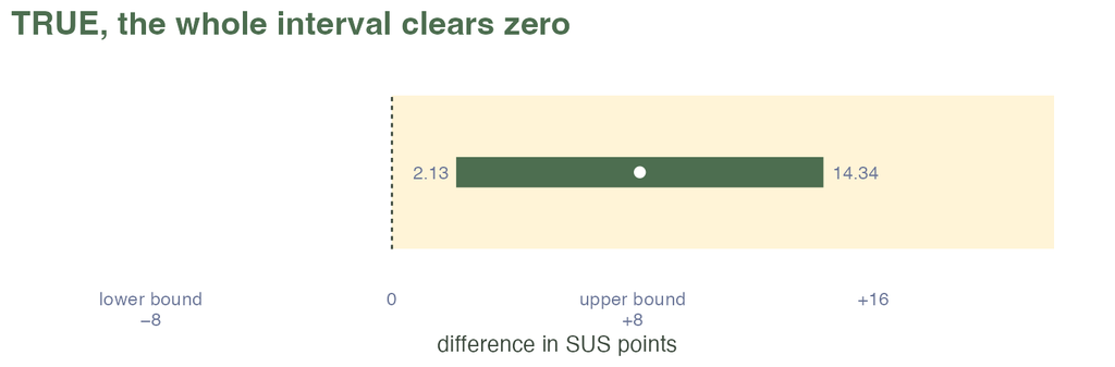
1. Against zero. We use the two-sided p-value at alpha .05.
fit$p.value # check p-value from our t-test
[1] 0.008583774

differs_from_zero <- fit$p.value < ALPHA # confirm and store outcome as boolean
differs_from_zero
[1] TRUE
The two-sided test rejects a zero difference at alpha .05. The 95% interval is [2.13, 14.34] SUS points.
2. Against the action-threshold values, we ask whether the 90% interval sits inside them. TOST contains two one-sided tests at alpha .05. Both must be rejected.
p_lower <- 1 - pt((difference + ACTION_THRESHOLD) / std_error, deg_free)   # is it above -ACTION_THRESHOLD?
p_upper <-     pt((difference - ACTION_THRESHOLD) / std_error, deg_free)   # is it below +ACTION_THRESHOLD?

inside_action_bounds <- max(p_lower, p_upper) < ALPHA # confirm and store outcome as boolean

inside_action_bounds
[1] FALSE
The result is FALSE. The study could not establish that effects at or beyond the action threshold are absent. This does not establish that the difference is big enough to act on. That is the next comparison.
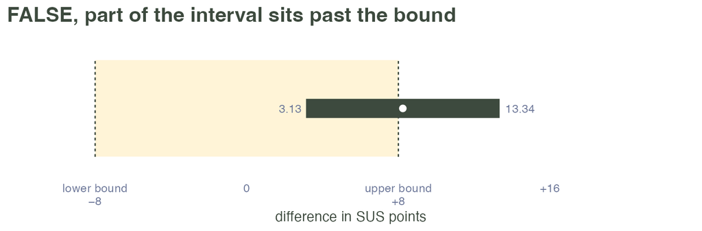
3. Against the action-threshold values, we ask whether the 95% interval sits beyond one of them. The minimum-effect comparison is a two-sided test, so it uses the 95% interval.
beyond_action_threshold <-  ci_95[1] > ACTION_THRESHOLD || ci_95[2] < -ACTION_THRESHOLD

beyond_action_threshold
[1] FALSE
The result is FALSE. The 95% interval does not fully clear either action threshold. The data do not establish a difference large enough to act on.
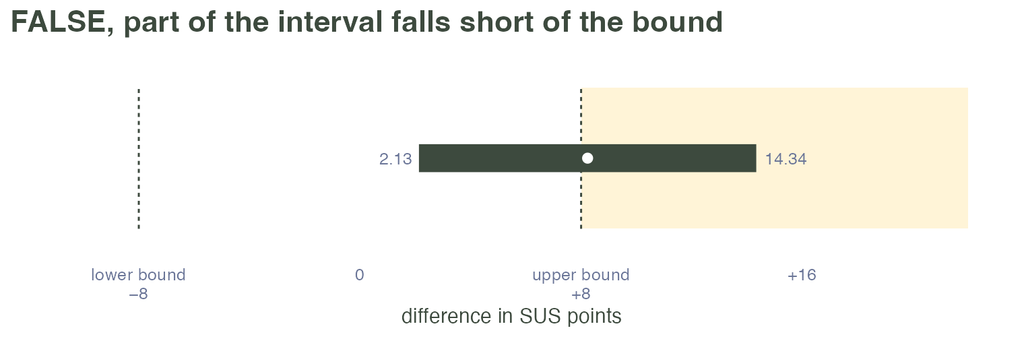
The example produces category B, the case that separates action-threshold testing from the Lewis and Sauro labels.
Those three comparisons combine into five possible states, depending on the data. We can pack that logic into an if/else statement. Note that order matters here. The code checks A first because every A result would otherwise also meet the broader condition for B.
verdict <- if (differs_from_zero && beyond_action_threshold) {
  "A  a meaningful effect is established"
} else if (differs_from_zero && !inside_action_bounds) {
  "B  an effect exists, size undetermined"
} else if (differs_from_zero && inside_action_bounds) {
  "C  real, and too small to matter"
} else if (inside_action_bounds) {
  "D  a meaningful effect is absent"
} else {
  "E  inconclusive"
}

> verdict
[1] "B  an effect exists, size undetermined"
The result is “an effect exists, importance undetermined.” In more literal terms, the redesign scored higher on SUS, and the data excluded zero. The study showed there is a difference but could not establish whether the population difference is below or beyond the action threshold.
Existing packages
We can do this whole process more succinctly with existing packages, specifically eqtesting. You still need to do the difference-from-zero comparison manually, which is the main statistical-significance comparison from our t-test.
install.packages("eqtesting")
library(eqtesting)

w <- t.test(redesign, current)

tst(estimate = unname(w$estimate[1] - w$estimate[2]),
    se       = w$stderr,
    ROPE     = ACTION_THRESHOLD,            # or c(lower, upper) for asymmetric bounds
    df       = w$parameter,    # omit for the normal approximation
    alpha    = 0.05)

> tst(estimate = unname(w$estimate[1] - w$estimate[2]),
+     se       = w$stderr,
+     ROPE     = ACTION_THRESHOLD,            # or c(lower, upper) for asymmetric bounds
+     df       = w$parameter,    # omit for the normal approximation
+     alpha    = 0.05)
Exact (equivalence) confidence intervals (ECIs) and three-sided testing (TST) results reported
If using for academic/research purposes, please cite the papers underlying this program:
Fitzgerald, J. (2025). The Need for Equivalence Testing in Economics. MetaArXiv. https://doi.org/10.31222/osf.io/d7sqr_v1.
Isager, P. & Fitzgerald, J. (2024). Three-Sided Testing to Establish Practical Significance: A Tutorial. PsyArXiv. https://doi.org/10.31234/osf.io/8y925.
$bounds
                                                      Lower Bound Upper Bound
95% TST confidence interval (for precision)              2.134136    13.34288
95% equivalence confidence interval (for conclusions)    3.127455    13.34288
95% classic confidence interval (for conclusions)        2.134136    14.33620

$test
                                              ROPE Lower Bound ROPE Upper Bound
Test: Estimate Bounded Above ROPE (Two-Sided)               -8                8
Test: Estimate Bounded Within ROPE (TOST)                   -8                8
Test: Estimate Bounded Below ROPE (Two-Sided)               -8                8
                                              t-statistic   p-value Relevant
Test: Estimate Bounded Above ROPE (Two-Sided)    0.076332 0.9392845        Y
Test: Estimate Bounded Within ROPE (TOST)        0.076332 0.5303577        N
Test: Estimate Bounded Below ROPE (Two-Sided)    5.269726 1.0000000        N

$conclusion
[1] "The significance of the parameter is inconclusive."
We get the same answer with a lot less input code. One label can be confusing: at alpha .05, the package’s 95% equivalence interval has the same endpoints as an ordinary 90% confidence interval. The package calls it 95% because each endpoint is a 95% one-sided confidence limit. Together, those endpoints form the ordinary two-sided 90% interval.
The package reports TST as inconclusive for this example, just like our manual results. The separate zero test makes that TST conclusion into outcome B because the 95% interval excludes zero (there is some effect).
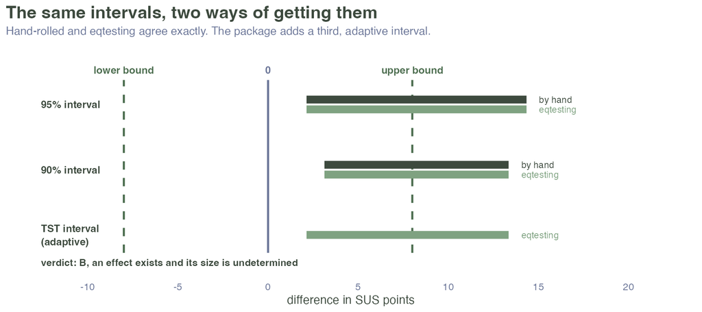
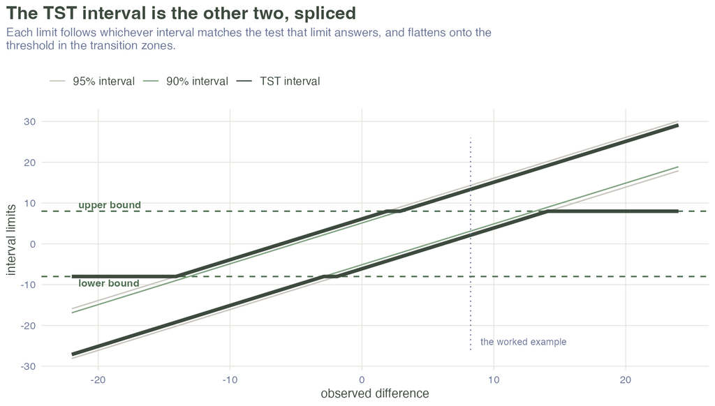
One benefit of eqtesting is an adaptive interval. In this example, the lower limit comes from the 95% interval and the upper limit comes from the 90% interval. Each limit corresponds to the relevant outward or equivalence comparison at that side of the estimate. The combination depends on the estimate’s location, so the same pair of limits will not apply to every result. This means you only need to report or visualize a single interval.
I’d suggest using eqtesting generally. On its own, the adaptive interval is easier to use than cross-comparing the separate intervals. These last (complex) charts are for people who want to inspect the logic behind the adaptive interval, but not something to share with stakeholders typically.
Summarizing our approach
This process is certainly complex if the ideas are brand new. Even in writing this all out, I learned a number of things in the process (+1 point for not letting AI write all your work for you). Coding the analysis lets you fix the decision rules ahead of time and rerun them consistently after the data arrive. Even if it takes a lot of time initially, you can reuse it on new projects quickly.
Let’s see what the process looks like in an overview for action-threshold testing in a cheat-sheet format.
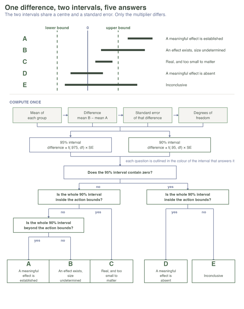
So in the end, we have a way to apply one consistent procedure that covers both statistical and practical significance. It gives us five possible outcomes that cover all the ways our comparison could go. In another post, I’ll get into some more complex worked examples if you want to see how this all might go outside of a simple SUS score.
More to come
The next post will get into how you should choose the action threshold. The choice requires evidence and individual judgment, but there are rigorous principles we can draw on. After that, we’ll talk about sample sizes. Using this procedure is more rigorous than simply inspecting one confidence interval, so it requires more power.
Wrap up
P-values come with established error-rate conventions and decision rules. Effect sizes have often come without such clear guidance. There is less convention to lean on, and the correct way to report an effect size is not fully settled. Isager and Fitzgerald, Goeman, Solari, and Stijnen, and Lakens have laid out repeatable ways to apply effect sizes alongside p-values.
Action-threshold testing gives a repeatable conclusion relative to a prespecified threshold, provided the model assumptions and threshold justification hold. You can implement the procedure in R and reuse the same code quickly on new projects.
As I said upfront, we started at the end: how to calculate results with an action threshold. The next post will dig into how you choose the threshold in the first place.
Appendix
Note: AI was used to support some research, coding, and visualization in this post.
Keep in mind that an action threshold may make less sense for exploratory studies. One counterargument is that a general baseline can still keep the team from making post hoc comparisons.
Footnotes
- NHST became a dominant frequentist practice during the twentieth century. I won’t cover it here, but this resource gives a useful introduction. ↩︎
- Lakens uses nil null hypothesis for a point value such as exactly zero. A non-nil null hypothesis contains a range of values. ↩︎
- Prespecification connects the Type I error rate to the decision rule. The confidence interval keeps its coverage. The post hoc label has no prespecified error rate because the result can influence what counts as close enough. ↩︎
- These are not independent tests that each add another chance of a false positive. They test connected regions of the same effect scale and are calibrated so that the chance of wrongly ruling out the region containing the true effect remains at the chosen alpha level. Imagine the possible true effects on one number line:
meaningfully negative | small negative | 0 | small positive | meaningfully positive
For any true effect, only one location on that line can be correct. These are not independent 5% chances.
If you apply the framework to several outcomes, segments, or model coefficients, you still need to address multiple comparisons across those relationships. ↩︎ - TST applies when the fitted model provides an estimate and standard error with a justified normal or Student-t reference distribution. The action bounds must use the same scale as the estimate. ↩︎
- The 90% and 95% intervals come from one fitted two-sample model. The procedure evaluates several prespecified hypotheses from that estimate.
wide <- t.test(redesign, current, conf.level = 0.95)narrow <- t.test(redesign, current, conf.level = 0.90)↩︎